How a Machine Learns

How a fly helped Descartes to invent the Cartesian plane

René Descartes (1596 – 1650), the famous philosopher and mathematician, was lying in his bed, eyes fixed on a fly on the ceiling.

As he pondered how to accurately describe the fly’s position, Descartes visualized the ceiling as a rectangle sketched on paper, using the bottom left corner as a starting point. To pinpoint the fly, one would simply measure the distance to travel horizontally and then vertically. These two numbers are the fly’s coordinates.

I can’t vouch for the authenticity of this tale. But what I do know is that the coordinate system he dreamt up, often referred to as the Cartesian plane, was nothing short of revolutionary. It seamlessly wove together Algebra and Geometry.

Learning functions and rate of change through a slice of bread

Suppose one slice of bread contains 100 calories. This can be represented algebraically as y = 100x, where x is the number of bread slices and y is the total calories from consuming x slices of bread. The graph below illustrates this equation visually.

x and y are variables where the value of x determines the value of y. We can consider x as an independent variable and y as a dependent variable. It can also be said that y is a function of x. A function is a set of rules that takes one or more inputs, applies the rule, and yields an output.

In the given example, the rule is to multiply the number of bread slices by 100 to determine the total number of calories. If you input 2, you get 200 calories. If you input 5, you get 500 calories. x and y have a linear relationship in this example.

In a linear relationship, the rate of change (slope) in y is consistent for every unit change in x. Each slice of bread produces 100 calories no matter how fast we eat. The slope is calculated as the change in y divided by the change in x, represented as Δy/Δx.

For example, if consuming 4 bread slices gives you 400 calories and 2 bread slices gives you 200 calories, the calorie increase per bread slice is calculated as (400 – 200) divided by (4 – 2), which equals 100.

The slope or rate remains constant at 100, whether you’re comparing between 6 and 8 slices or any other two points on the x-axis. This is the reason why you see a horizontal line at 100 on the right chart above. Although the rate is represented by the number 100, it’s technically a function. Rate is a constant function in the bread slice example. Steven Strogatz, in his insightful book “Infinite Powers,” elaborates this idea.

When a rate is constant, it’s tempting to think of it as simply being a number, like 200 calories per slice or $10 an hour or a slope of 1/12. That causes no harm here, but it would get us into trouble later. In more complicated situations, rates will not be constant. For example, consider a walk through a rolling landscape, where some parts of the hike are steep and others are flat. On a rolling landscape, slope is a function of position. It would be a mistake to think of it as a mere number. Likewise, when a car accelerates or when a planet orbits the sun, its speed changes incessantly. Then it’s vital to regard speed as a function of time. So we should get in that habit now. We should stop thinking of rates of change as numbers. Rates are functions.

Nonlinear functions and the idea of a derivative

However, not all functions in nature are linear. When a function is not linear, its rate of change, Δy/Δx, is not constant. Consider the nonlinear function s = t². It describes the position change of “s” an object as a function of “t”.

The graph on the left tracks the object’s position over time. s = t² is a nonlinear function, and its graph is a curve, unlike the straight line we observed in the bread slice example. The graph on the right tracks the rate of change of position over time, which is also known as velocity. The change in velocity is represented by a slanted line, in contrast to the horizontal line we saw in the bread slice example.

What is the velocity of the object at t = 4 seconds?

It might be tempting to use the slope formula we applied for linear function here, but that would yield the average velocity between t1 and t2 seconds. For instance, the first triangle on the left chart calculates the average velocity using the formula (5² – 3²) / (5 -3), resulting in an average velocity of 8 m/s.

The second triangle on the left chart calculates the average velocity using the formula (9² – 7²) / (9 -7), resulting in an average velocity of 16 m/s. The velocity differs between these two points. Moreover, if you select any pairs of points on the curve, you’ll discover that each has a unique velocity.

The question is not about calculating average velocity, but rather instantaneous velocity. Think of this as looking at the speedometer to find out how fast the car is traveling at a particular moment.

What if we set t1 and t2 to 4 seconds? (4² – 4²) / (4 – 4). That won’t work as dividing by zero is forbidden.

In the 17th century, Newton and Leibniz developed calculus to address challenges posed by variables that shift continuously over time. They understood that their existing tools were apt for linear functions but fell short for nonlinear functions involving constant change.

They found that if you keep narrowing in on a curve, it will ultimately resemble a straight line. But there’s a catch: the increase in ‘x’ must be infinitesimally tiny. This insight allowed them to apply the conventional slope formula.

If we set the infinitesimally small amount to 0.00001 and do (4.00001² – 4²) / (4.00001 – 4), we obtain a result of 8 m/s. This method is known as taking the derivative. I set t = 4 and got the derivative as 8 m/s. Obviously, this method isn’t scalable as the velocity is different for each value of t.

Mathematicians are smart. They abstract everything and provide us a simple formula to use to calculate the derivative on any point we want. For a t² function the derivative is 2t. This is the reason why we got the derivative of 8 m/s at t = 4s (2 * 4). It’s easy to derive why the derivative of t² is 2t  through first principles.

What can we learn from the magnitude and direction of a derivative?

Derivatives offer two essential pieces of information, paving the way for machine learning. Take a look at the graph for a nonlinear function y = x². I made four points p1, p2, p3, and p4 on it. Each point provides us the magnitude and direction of how the y value is changing with respect to x.

At point P1, where x is -8, y is 64, and the derivative is -16. What does the negative sign tell you? As x increases, for instance from -8 to -7, the value of y decreases from 64 to 49. A similar trend is observed at point P2.

Let’s disregard the sign for now. What does the magnitude of 16 at P1 indicate? The value of y changes significantly more when the magnitude is higher compared to when it’s lower. As x increases from -8 to -7, the value of y decreases from 64 to 49. In contrast, when x rises from -3 to -2, the value of y drops from 9 to 4—a much smaller change since the magnitude at P2 is less than that at P1.

At point P3, the value of the derivative is 0. This suggests that the value of y is at its minimum when x is 0.

At point P4, where x is 3, y is 9, and the derivative is 6, a positive sign indicates that y increases as x increases. By understanding both the magnitude and the direction (sign) of the derivative, we can predict how the value of y changes as x changes. This predictive capability is profound, and machines utilize it to learn.

Let’s make the machine predict weight based on height

I’ve created a simple weight function that accepts height in centimeters as input and calculates the weight using the formula 0.32 * height. To introduce variability, I’ve added a random noise of up to 15% to the weight.

For instance, if the weight is 100 kgs and the noise factor is 0.15, the noise can range from -15 kgs to 15 kgs. This means the resulting weight can vary between 85 kgs and 115 kgs. I generated weights for 100 random heights ranging from 150 to 190 cm and displayed the results in the scatterplot below.

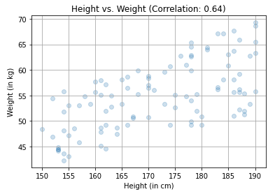
The machine isn’t aware of the formula I used to generate the data. Can we input the height and weight data into the machine, allowing it to construct a model that understands the correlation between height and weight, and then predict the weight for new heights?

The model will try to come up with the best value for height_coefficient so that its weight prediction (height_coefficient * height) comes as close as possible to the actual weight. Let’s assume that we train the model with one example with a height of 161 cm and a weight of 47.81 kgs.

Assume that the model initializes the height_coefficient with a random value set to 0. With this, its predicted weight will be zero (since 0 multiplied by 161 equals 0). To evaluate the quality of the model’s prediction, we can create a loss function. This function squares the difference between the predicted weight and the actual weight. In this case, the squared difference is (0 – 47.81)², which equals 2286.

I graphed the relationship between height_coefficient and the loss function below. The objective of the model is to adjust the height_coefficient so that the value for the loss function is close to zero. When does the loss value get close to zero? It happens when the model prediction gets closer to actual value.

By taking the derivative of the loss function with respect to the height_coefficient, we can determine how much to increment or decrement the height_coefficient in order to reduce the loss. The derivative of the loss function is given by: 2 * height * (height_coefficient * height – actual_weight).

When we substitute the given values, 2 * 161 * (0 * 161 – 47.81), the resulting value of the derivative is -15,394.82. What does the negative sign indicate? It suggests that if you increase the height coefficient, the value of the loss will decrease.

How much should we adjust the height coefficient? We shouldn’t directly use the value of -15,394.82. Instead, we should apply a smaller amount to ensure we gain insights gradually from a specific example. This approach prevents us from overly relying on one example.

This adjustment is known as the learning factor, and I’ve chosen 0.00001 as its value. When we multiply -15,394.82 by 0.00001, we get -0.15. The table below captures all the computations discussed after the first iteration.

Iteration	Height	Height Coefficient	Predicted weight	Actual weight	Loss	Derivative	Learning rate	Add to Height coefficient	Updated Height Coefficient
1	161	0	0	47.81	2286.14	-15395.97	0.00001	0.15	0.15

The last column “Updated Height Coefficient” will be the new height coefficient used by the model for the next iteration. I was able to bring the loss close to zero on this one example with a height coefficient reaching 0.29.

Iteration	Height	Height Coefficient	Predicted weight	Actual weight	Loss	Derivative	Learning rate	Add to Height coefficient	Updated Height Coefficient
1	161	0	0	47.81	2286.14	-15395.97	0.00001	0.15	0.15
2	161	0.15	24.79	47.81	530.20	-7414.39	0.00001	0.07	0.23
3	161	0.23	36.72	47.81	122.96	-3570.62	0.00001	0.04	0.26
4	161	0.26	42.47	47.81	28.52	-1719.54	0.00001	0.02	0.28
5	161	0.28	45.24	47.81	6.61	-828.10	0.00001	0.01	0.29

I trained the model using all 100 heights and weights. It converged to a height_coefficient of 0.32 after 15 iterations. It predicts the right weight of 52 kgs for 162 cm height. The chart below shows how the loss fell close to zero while the height_coefficient went up to 0.32.

Congratulations! We’ve successfully trained the model to predict the correct weight. The modeling technique we used is called Linear Regression. The type of training is supervised training as we had to prepare the training data. The model came up with a line fit that approximated the input data.

You don’t need to write a lot of code

I recently came across a thought-provoking statement by Andrew Ng, a renowned figure in the AI world. He mentioned, “An individual fluent in multiple languages — for instance, having English as their primary language and Python as their secondary — has a greater potential than one who merely knows how to interact with a large language model (LLM).” Andrew’s perspective resonates deeply with me.

I highly recommend working on 3 best books I have come across to get fluent in Python, develop the mental models necessary to work with n-dimensional data, and grok the foundations of machine learning. Python Distilled, Python for Data Analysis, and Programming Machine Learning are those 3 books.

How many lines of code do you estimate it took to train this basic model? In reality, it required only 22 lines. Given below is the code with annotations added to aid readability.

The derivative is one of the most important concepts to understand deeply. It’s like the gateway to the world of machine learning. I would highly recommend reading Chapter 8: Understanding rates of change from the book Math for Programmers.

Height is one parameter, but the model could be enhanced with additional ones. This requires minor adjustments to the Python code, specifically for doing partial derivatives, matrix multiplication and transpose. I’ll discuss this in my next post.